杜老师课程学习记录，仅供个人学习使用，模型TensorRT部署之前的前处理和后处理分析，python简单实现。

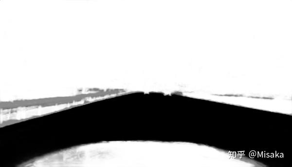
路面分割模型

查看模型onnx文件，获得模型的输入输出维度：

输入维度：[1,3,512,896]
输出维度：[1,512,896,4]

模型是一个全卷积网络，输入和输出大小相同，不管模型多么复杂，先分析前处理和后处理，先用python实现。

预处理：标准化->cv2.resize()->维度切片->astype(np.float32)

源代码是直接使用的BGR格式，也不需要仿射变换。

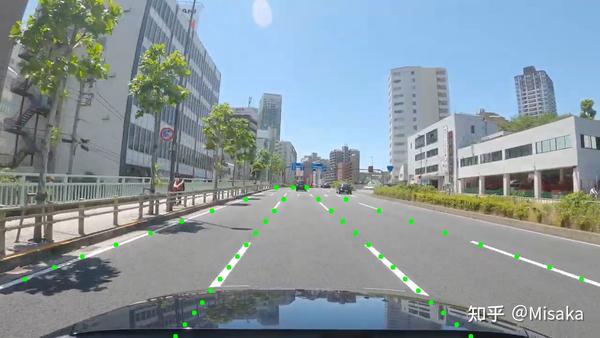
车道线检测模型

输入维度：[1, 3, 288, 800]
输出维度：[1, 201, 18, 4]

用到的算法是Ultra-Fast-Lane-Detection，和熟悉的yolo系列检测算法还不太一样，Ultra-Fast-Lane-Detection是基于位置概率实现的。首先将连续的车道线离散成点，通过若干个点去表示车道线，因此问题转化为预测点的坐标，根据先验车道线肯定在路面上，而且在图片的下半部分，那么预先在图像高度方向上划分出若干条线，例如该模型是预先在高度方向上画18条线，即每条车道线会由18个点表示，并且18个点的y坐标已经确定好了，因此预测点(x, y)坐标转化成了只需要预测x坐标问题。

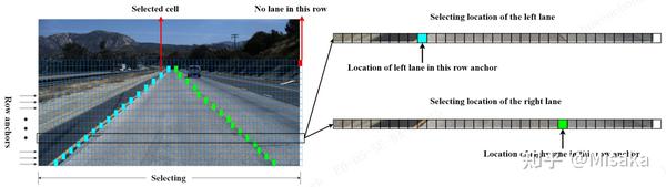
然后通过位置概率获得x坐标值，大概可以理解为：按图像的宽度方向，把图像分为若干个位置，比如该模型是把图像宽度分成了200个位置，再加上一个点不在图像上位置，那么总共就是201个位置，每个位置模型会输出一个位置概率，即表示点落在该区域的概率，因此模型输出维度[1, 201, 18, 4]，可以理解为：201个位置概率（宽度方向格子数），一条车道线由18个点表示（y轴方向上的划线数），4表示业务场景只存在4条车道线。

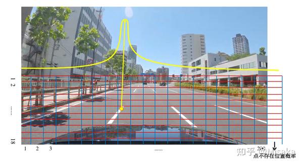
那么如何通过模型结果得到x坐标：首先对模型输出结果在201这个维度上计算softmax()，获得位置概率 O_{probability}，然后位置编号点乘位置概率 O_{probability}后相加得到 O_{mul} ，再判断位置概率O_{probability}最大的位置是否是200(对应图像上的201，即点不存在的情况)，如果是，表示点不存在，将O_{mul}中对应索引元素置为0，即过滤该点。

预处理步骤：
cv2.resize(image, (288, 800))，这里注意的是直接resize，刚开始以为是裁剪图像，只保留图像的下半部分，发现输出结果不对。
BGR->RGB
标准化并转化为np.float32
维度切片：(1, height, width, 3)->(1, 3, height, width)
后处理步骤：
模型输出的维度其实是：(1, 1, 201, 18, 4)
对201维度进行softmax()，得到位置概率O_{probability}
位置概率和位置编号点乘，之后求和得到O_{mul}，O_{mul}维度为(18, 4)
判断位置概率O_{probability}最大的位置是否是200，如果是，将O_{mul}中对应索引元素置为0。
后处理可以直接写进onnx，可以省略C++代码编写量。

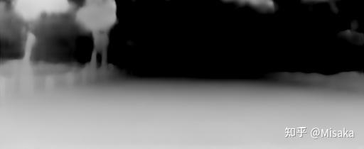
深度估计

输入维度：[1,3,256,512]

输出有六个，估计是全卷积网络反卷积过程的每个阶段都输出了，使用时取最后一个就好了，维度为[1, 1,256,512]

预处理：cv2.resize()->(BGR->RGB)->标准化->维度切片和np.float32

后处理：源代码中有个裁剪操作，把图像上面的18%裁剪掉了，并且对输出结果out*(-5)+255，便于可视化。

import cv2
import numpy as np
import onnxruntime
import matplotlib.pyplot as plt
import scipy
'''
预处理和后处理步骤：
1：路面分割
    预处理：
    标准化：normalize=(image-mean)*norm
    输入图像尺寸：不需要仿射变换，直接resize，512*896
    输入图像格式：BGR
    np.float32
    输出图像通道：4通道

2:车道线检测
    预处理：
    cv.resize
    标准化
    BGR->RGB
    np.float32
    输出维度：1*1*201*18*4，201表示位置，18表示车道线由18个点表示，4表示有4根车道线
    后处理：
    201维度：softmax
    点乘相加
    200位置点 out_j置0

3：深度估计
    输入[1,3,256,512]
    输出有6个，估计是全卷积网络反卷积过程的每个阶段都输出了
    使用时取最后一个就好
    前处理：
    resize()
    BGR->RGB
    标准化
    切片和np.float32
    后处理：
    裁剪
    out *（-5）+ 255
'''

#路面分割
def loadSegment(onnxFile, imgFile, size):
    width, height = size
    oriImg = cv2.imread(imgFile)
    image = cv2.resize(oriImg, size).astype(np.float32)
    #ascontiguousarray()内存不连续的数组，变为连续的数组，加快运行速度
    imgTensor = np.ascontiguousarray(image.transpose(2,0,1).reshape(-1,3,height, width))
    sess = onnxruntime.InferenceSession(
        onnxFile,
        providers=["CPUExecutionProvider"]
    )

    input_name = sess.get_inputs()[0].name
    output = sess.run(None, {input_name: imgTensor})
    out = output[0][0].transpose(2,0,1)
    cv2.imwrite("segment.jpg", out[0]*255)

#车道线检测
def UltraFastLaneDetection(onnxFile, imgFile, size):
    mean = np.array([0.485, 0.456, 0.406])
    std = np.array([0.229, 0.224, 0.225])
    width, height = size
    oriImg = cv2.imread(imgFile)
    # image = oriImg[-288:, :, :]
    image = cv2.resize(oriImg, size)

    image = cv2.cvtColor(image, cv2.COLOR_BGR2RGB)
    image = image/255.0
    image = (image - mean)/std
    image = image.astype(np.float32)
    imgTensor = image.reshape(-1, height, width, 3).transpose(0,3,1,2)
    print(imgTensor.shape)

    sess = onnxruntime.InferenceSession(
        onnxFile,
        providers=["CPUExecutionProvider"]
    )
    input_name = sess.get_inputs()[0].name
    output = sess.run(None, {input_name: imgTensor})
    print(np.array(output).shape)

    # 打印结果
    out = np.array(output[0])[0]
    griding_num = 200
    col_sample = np.linspace(0, 800 - 1, griding_num)
    col_sample_w = col_sample[1] - col_sample[0]

    out_j = out
    out_j = out_j[:, ::-1, :]
    prob = scipy.special.softmax(out_j[:-1, :, :], axis=0)
    idx = np.arange(griding_num) + 1
    idx = idx.reshape(-1, 1, 1)
    loc = np.sum(prob * idx, axis=0)
    out_j = np.argmax(out_j, axis=0)
    print(out_j)

    loc[out_j == griding_num] = 0
    out_j = loc

    row_anchor = [121, 131, 141, 150, 160, 170, 180, 189, 199, 209, 219, 228, 238, 248, 258, 267, 277, 287]
    cls_num_per_lane = 18
    img_w, img_h = oriImg.shape[1], oriImg.shape[0]

    for i in range(out_j.shape[1]):
        if np.sum(out_j[:, i] != 0) > 2:
            for k in range(out_j.shape[0]):
                if out_j[k, i] > 0:
                    ppp = (int(out_j[k, i] * col_sample_w * img_w / 800) - 1,
                           int(img_h * (row_anchor[cls_num_per_lane - 1 - k] / 288)) - 1)
                    cv2.circle(oriImg, ppp, 5, (0, 255, 0), -1)

    cv2.imwrite("ultra-lane-draw.jpg", oriImg)

#深度估计
def ldrn(onnxFile, imgFile, size):
    mean = np.array([0.485, 0.456, 0.406])
    std = np.array([0.229, 0.224, 0.225])
    width, height = size
    oriImage = cv2.imread(imgFile)
    image = cv2.resize(oriImage, size)
    image = cv2.cvtColor(image, cv2.COLOR_BGR2RGB)
    image = image/255.0
    image = (image - mean) / std
    image = image.astype(np.float32)
    imgTensor = image.transpose(2,0,1).reshape(1, 3, height, width)

    sess = onnxruntime.InferenceSession(
        onnxFile,
        providers=["CPUExecutionProvider"]
    )
    input__name = sess.get_inputs()[0].name
    output = sess.run(None, {input__name: imgTensor})
    print(np.array(output[5]).shape)

    out = np.array(output[5]).reshape((256, 512))
    # 源代码中有个裁剪和*(-5) - 255的操作，给它加上
    out = out[int(out.shape[0] * 0.18):, :]
    out = out * -5 + 255
    plt.imshow(out)
    plt.show()
    # cv2.imwrite("ldrn.jpg", out)

if __name__ == "__main__":
    segFile = "road-segmentation-adas.onnx"
    # ultraFile = "ultra_fast_lane_detection_culane_288x800.onnx"
    # ldrnFile = "ldrn_kitti_resnext101_pretrained_data_grad_256x512.onnx"
    imgFile = "dashcam_00.jpg"

    loadSegment(segFile, imgFile, (896,512))
    # UltraFastLaneDetection(ultraFile, imgFile, (800, 288))
    # ldrn(ldrnFile, imgFile, (512, 256))